Microsoft Excel: Spreadsheet Optimization Strategies
Microsoft Excel is a powerful tool for data analysis and manipulation. However, spreadsheets can quickly become unwieldy and inefficient if they are not properly optimized. By following a few simple optimization strategies, you can improve the performance and usability of your spreadsheets.
1. Use a Separate Worksheet for Each Table
One of the most common mistakes people make when creating spreadsheets is to put all of their data on a single worksheet. This can make it difficult to find the data you need and can also lead to performance problems.
Instead, it is better to use a separate worksheet for each table of data. This will make it easier to organize your data and will also improve performance.
2. Use Named Ranges
Named ranges are a great way to make your spreadsheets more readable and easier to use. A named range is simply a range of cells that has been given a name. You can then use the name of the range in formulas and other spreadsheet functions.
To create a named range, select the range of cells you want to name and then click on the "Formulas" tab. In the "Defined Names" group, click on the "Create From Selection" button. In the "Create Name" dialog box, enter a name for the range and then click on the "OK" button.
3. Use Formula Auditing Tools
Excel has a number of built-in formula auditing tools that can help you find and fix errors in your formulas. These tools include the "Formula Evaluator" and the "Trace Precedents" and "Trace Dependents" commands.
To use the Formula Evaluator, select the formula you want to evaluate and then click on the "Formulas" tab. In the "Formula Auditing" group, click on the "Evaluate Formula" button. The Formula Evaluator will show you the value of the formula at each step in its calculation.
To use the Trace Precedents and Trace Dependents commands, select the cell that contains the formula you want to trace and then click on the "Formulas" tab. In the "Formula Auditing" group, click on the "Trace Precedents" or "Trace Dependents" button. Excel will highlight the cells that are used in the formula or that are affected by the formula.
4. Use Conditional Formatting
Conditional formatting is a great way to make your spreadsheets more visually appealing and easier to read. Conditional formatting allows you to apply different formatting to cells based on their values.
For example, you could use conditional formatting to highlight cells that contain errors or to show the top or bottom performers in a data set.
5. Use Macros
Macros are a great way to automate repetitive tasks in Excel. A macro is a set of instructions that you can record and then play back later.
Macros can be used to perform a wide variety of tasks, such as formatting data, creating charts, or sending emails.
By following these simple optimization strategies, you can improve the performance and usability of your spreadsheets. This will make it easier to find the data you need and will also help you avoid errors.